This is the second part of the deep dive into my Formula One model. Part I provided a high-level overview of the approach. Today's post will go into the details of the implementation, how the model calculates reliability and performance for both teams and drivers, and allocates results to each. Future posts will outline how the knobs are tuned, evaluate its predictive power, and walk through how the predictive ratings are aggregated into backwards-looking "resume" ratings like the ones used in the 2021 preview.
Calculating Reliability
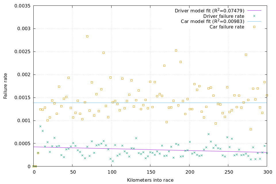
As stated in the previous post, the goal of our reliability model is to predict the odds of failure in an average kilometer for each car and for each driver. The model tracks reliability in five buckets:
- Per-driver reliability (ability to not crash);
- Aggregate reliability of all drivers in the field;
- Per-team reliability;
- Aggregate reliability of "mature" teams in the field; and
- Aggregate reliability of "new" teams in the field.
These are measured in terms of “success kilometers” and “failure kilometers”. The probability of per-kilometer success of a car or driver is simply [(success kilometers) / (total kilometers)]. Since the probability of success each kilometer is independent of the previous kilometer, the probability of a car not suffering a mechanical DNF in an X-km race is the per-kilometer car success probability raised to the Xth power; the same calculation is also done using the driver per-kilometer success probability. Since driver-related DNFs are independent of car-related DNFs, the probability of an entrant successfully completing the whole race distance is (car success probability * driver success probability).
We separate out the "new" team reliability from the "mature" team reliability due to the chaotic nature of the early days of Formula One. There have been just shy of 500 unique teams to take part in F1 over the decades. Of those, around 300 joined in the 1950s, another 100 joined in the 1960s, and the rest started their lineage in 1970 or later. While there is a big gap between today's "haves" and "have-nots", the gap was noticably larger in the early days of the sport. For example, the 1953 German Grand Prix alone had more one-race teams-slash-privateers-as-constructors (Dora Greifzu, Rennkollektiv EMW, Ernst Loof, Erwin Bauer, Gunther Bechem, Oswald Karch, and Rodney Nuckey) than truly new teams have joined Formula One in the last 20 years (Toyota, Super Aguri, HRT, Team Lotus, Virgin, and Haas).
For each entrant there are three possible outcomes in an X kilometers long race. If the entrant:
- completes the entire race distance, we update the number of success kilometers for four buckets -- the first three buckets plus one for either the "new" or "mature' team -- by X;
- completes Y kilometers but then suffers a mechanical DNF, we:
- add Y success kilometers to those four buckets; and
- add a small constant in the range [0, 1] to the number of failure kilometers for the two relevant team-related buckets (team_reliability_failure_constant);
- completes Z kilometers but then suffers a driver-attributed DNF, we:
- add Z success kilometers to the four relevant buckets; and
- add a small constant in the range [0, 1] to the number of failure kilometers for the two driver-related buckets (driver_reliability_failure_constant).
The driver_reliability_failure_constant and team_reliability_failure_constant parameters allow us to hone in on the best ratios to predict driver and car failure.
Before adding the results of the current race to any of the buckets, we apply a decay factor to the existing data (driver_reliability_decay or team_reliability_decay) to gradually age out existing data.
Before the first race of each season we regress the aggregate "new" team reliability back to the "mature" team reliability by a certain amount. Before the first race a driver or team participates in in a new season, we regress their reliability back to the mean by a fixed percent (driver_reliability_regress and team_reliability_regress). Whether we regress the team to the "new" or "mature" bucket depends on the number of races in which the team has participated. At this point we also cap the total kilometers in their reliability data set to a fixed multiple of an average race distance (driver_reliability_lookback and team_reliability_lookback). This makes the reliability metrics slightly more sensitive to change during the earlier stages of the season.
When a new driver or team appears for the first time, we give them the default reliability rate of the entire field.
While we could use an existing implementation of a Kaplan-Meier survival estimator or an exponential survival model in something like Scikit or Lifelines, these approaches are heavyweight and did not produce a statistically superior predictor. Additionally, they increased the runtime of our model from ~90 seconds to 30 minutes (Kaplan-Meier) or 180 minutes (exponential survival).
Calculating Performance
Performance is calculated using a hybrid Elo model, in which drivers and teams are modeled independently and then combined for each entrant. Elo ratings are updated for each entrant after each qualifying session, and in races only if an entrant does not suffer a driver-related or car-related DNF.
New drivers start with driver_elo_initial points, and new teams with team_elo_initial points.
Car vs Driver
The combined entrant rating and K-Factors are calculated using a weighted average of the driver Elo information and the car (team) Elo information. This weighting can change over time, and is specified by the team_share_spec parameter. The parameter is specified as [InitialTeamShare]_[YearWidth]_[StepHeight], where InitialTeamShare is the percent of the entrant Elo information coming from the car in 1950 (the first season), and then every YearWidth seasons that number will increase by StepHeight percent. For example, a spec of 50_4_1 means that from 1950 through 1953, the team contributes 50% of the Elo information to the entrant Elo information, then from 1954 through 1957 it contributes 51%, 1958 through 1961 is 52%, and so on. A spec of [N]_0_0 signals a constant share of N% throughout the history of Formula One. This allows us to empirically test the hypothesis that the share of overall results due to the car has steadily increased over time, without risking overfitting on a per-season basis.
We apply this weighted average between car and driver to both the Elo rating and K-Factor when creating the combined Elo information. For example, in a season where the car accounts for 60% of the outcome, a combination of the following car and driver would produce these combined Elo and K-Factor ratings:
| Car | Driver | Combined | |
|---|---|---|---|
| Elo | 1260 | 1560 | 756 + 624 = 1380 |
| K-Factor | 13 | 18 | 7.8 + 7.2 = 15.0 |
This gives us the basic combined Elo rating and K-Factor of the entrant.
Starting Position Advantage
For races (but not qualifying) we must also take into account starting position on the grid. The model treats starting position much like home field advantage, in that it will give the driver closer to the front of the grid a boost in their Elo ratings for that one head-to-head prediction. It is likely that this advantage is non-linear, meaning that at some point there is no significant difference between starting N positions ahead of another entrant versus N+1 positions ahead; e.g., there may be a noticeable difference between having a 2 space advantage versus a 5 space advantage, but less difference between 12 spaces and 15 space. It is also possible that the base advantage of a single grid spot has increased over time, contributing to the sense that Formula One races are glorified parades.
We model this advantage through a combination of two parameters:
- position_base_spec: formatted the same as team_share_spec, this allows us to vary the number of Elo points a single grid spot confers as an advantage over time; and
- position_base_factor: a value used as the ratio for a geometric sum, mapping the number of grid positions to a multiplier of the base spec for that year.
Plugging all this into the geometric sum formula, the Elo advantage EA conferred by G grid positions in a season with a base Elo grid advantage of EB and a factor of F is:
EA = EB * [(1 - FG) / (1 - F)]
The values of the base advantage and the base factor control the shape of the curve for this advantage. Values of F closer to 1 create a more linear shape, while lesser values create a flatter shape.

Predicting Performance Outcomes
Once we have the combined Elo rating and (for races) the start position advantage, we can then use these numbers to predict the probability that one entrant will finish in front of another entrant (assuming both finish) using the expected score logistic equation.
For this equation, though, we need to determine the correct denominator. From the Wiki page, a denominator of 400 means that “for each 400 rating points of advantage over the opponent, the expected score is magnified ten times in comparison to the opponent's expected score”. Or, in terms of odds, a denominator of X means that an Elo rating advantage of X points represents a 10-to-1 favorite, whereas a rating advantage of 2X points represents a 100-to-1 favorite.
Since qualifying is shorter and has less variance, we may expect that the same performance difference in qualifying would yield greater odds of winning than the same performance difference in a race. The model allows us to specify elo_exponent_denominator_qualifying and elo_exponent_denominator_race separately in order to keep the Elo rating constant between event types, but still capture the differences in these types.
Combined Head-to-Head Model
Putting this all together the probability that driver A in car X finishes (entrant E) ahead of driver B in car Y (entrant F) is:
- the probability that entrant E finishes the race but F does not (the car and driver reliability calculations); plus
- the probability that entrant E does not finish the race but completes more laps than F (per-lap reliability calculations); plus
- conditional on both E and F completing the race, the probability that E outperforms F (performance calculations).
Of those, the second is the most complex to calculate, but contributes the least to the final probability.
If both entrants complete the race (or participate in the qualifying session) we must reallocate Elo points. The K-Factor used for any transfer of points is the average of the combined K-Factor for each entrant. The Elo rating for each entrant is the combined Elo rating of each entrant, plus the starting position advantage points for whichever entrant starts first.
For example, let's say that there are four entrants which complete a race, two teams of two drivers each. In this year the car accounts for 60% of the performance, the base Elo advantage for one grid spot is 20 points, and the position factor is 0.75.
The two teams:
| Team | Elo | K-Factor | Reliability |
|---|---|---|---|
| X | 1400 | 16 | 93% |
| Y | 1350 | 20 | 91% |
The four drivers:
| Driver | Elo | K-Factor | Reliability |
|---|---|---|---|
| A | 1400 | 12 | 98% |
| B | 1300 | 20 | 90% |
| C | 1525 | 10 | 95% |
| D | 1350 | 16 | 91% |
The four entrants, in grid order:
| Entrant | Elo | K-Factor | Reliability | Grid |
|---|---|---|---|---|
| E: A+X | 1400 | 14.4 | 91.1% | 1 |
| G: C+Y | 1420 | 16.0 | 86.4% | 2 |
| H: D+Y | 1350 | 18.4 | 82.8% | 3 |
| F: B+X | 1360 | 17.6 | 83.7% | 4 |
The head-to-head performance-only probabilities, assuming an Elo denominator of 240:
| Entrant 1 | Entrant 2 | E1 | |||
|---|---|---|---|---|---|
| Name | Elo | Grid | Name | Elo | WinProb |
| E | 1400 | 20 | G | 1420 | 50.0% |
| E | 1400 | 35 | H | 1350 | 69.3% |
| E | 1400 | 46 | F | 1360 | 69.5% |
| G | 1420 | 20 | H | 1350 | 70.3% |
| G | 1420 | 35 | F | 1360 | 71.3% |
| H | 1350 | 20 | F | 1360 | 52.4% |
Note that without the one spot grid advantage for E over G, G would be the slight favorite, whereas on performance now it's a dead heat.
The probabilities above are also conditional on both entrants finishing. Digging into the E vs G matchup a bit more, there are the following scenarios, along with the probability that E finishes ahead of G:
| Scenario | P(happening) | P(E wins) if this happens |
P(E wins) total |
|---|---|---|---|
| Both finish | 78.7% | 50.0% | 39.4% |
| E finishes G DNFs |
12.4% | 100.0% | 12.4% |
| E DNFs G finishes |
7.7% | 0.0% | 0.0% |
| Double DNF | 1.2% | 50% | 0.6% |
| Overall | 52.4% | ||
Putting it all together, a much quicker driver becomes the slight underdog against an average-yet-reliable driver in a solid-but-slightly-more-reliable car who's managed to qualify on pole.
Coming up...
Part III will discuss its predictive performance. Part IV will discuss how predictions get aggregated into metrics which span one or more year.